Activity 06

NLP for GIS

From naturally processing language to natural langauge processing

Before 11:59pm on Wednesday, 4/16, you should submit to Canvas: * A document in pdf or docx format, answering all the questions in green boxes, and which are summarized in the deliverables section * A screenshot in that document of your geocoded and symbolized data in QGIS

Introduction and context

In this activity, you’ll geocode historical address data. In this case, you’ll work with data from the 19th century American children’s book trade directory. The directory contains 2,600 entries documenting the activity of individuals and firms involved in the manufacture and distribution of childrens books in the United States chiefly between 1821 and 1876. It’s searchable online, and—more importantly for us—you can download the data from the University of Pennsylvania’s Scholarly Commons.

The major difference between this activity and previous ones is that you’ll be using a different geographic information system: QGIS!

QGIS is a powerful, free, and open-source GIS software. You can do lots of the things in QGIS that you can do in ArcGIS Pro, including sophistiated vector and raster visualization/analysis.

QGIS is available on the Data Lab computers. Part of this activity will involve teaching yourself how to use it—now that you know your way around ArcGIS Pro, the learning curve for this will be less steep.

If you’re unsure how to do something in QGIS—for example, adding vector data—your first step should be to just Google it (e.g., qgis load vector data). We also have a guide from the Leventhal Center on getting started with QGIS, which may come in handy. There are also a ton of resources on getting started with QGIS from Tufts.

Set up your workspace

Directory stuff

You know what works for you. Set up a workspace for this activity!

Open QGIS!

Open QGIS by typing “QGIS” into the search bar at the bottom left-hand side of the screen. Click the application when it appears.

When it opens, you’ll be invited to start a “New empty project.” Go ahead and double-click it:

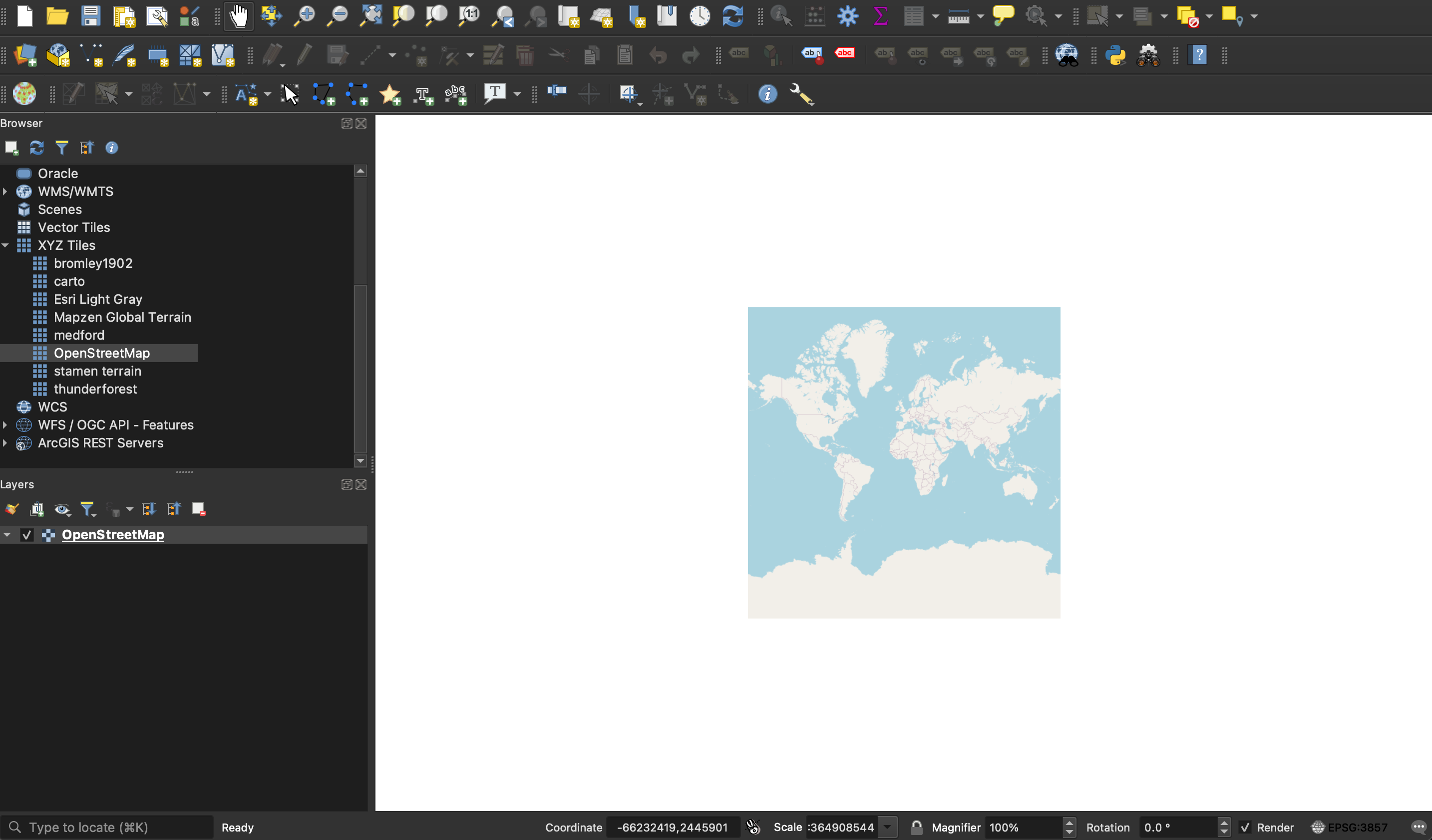
Once you’re in QGIS, the interface should look fairly familiar. Here are the main components:

In the Browser panel, double-click “XYZ tiles” and then double-click “OpenStreetMap”. This should add an OpenStreetMap base map layer to your map canvas, and a layer will appear in the layers list underneath the browser panel:

Now that you’ve got a working project, save the file in your workspace before moving on to the next step.

Getting the data ready

Download the data

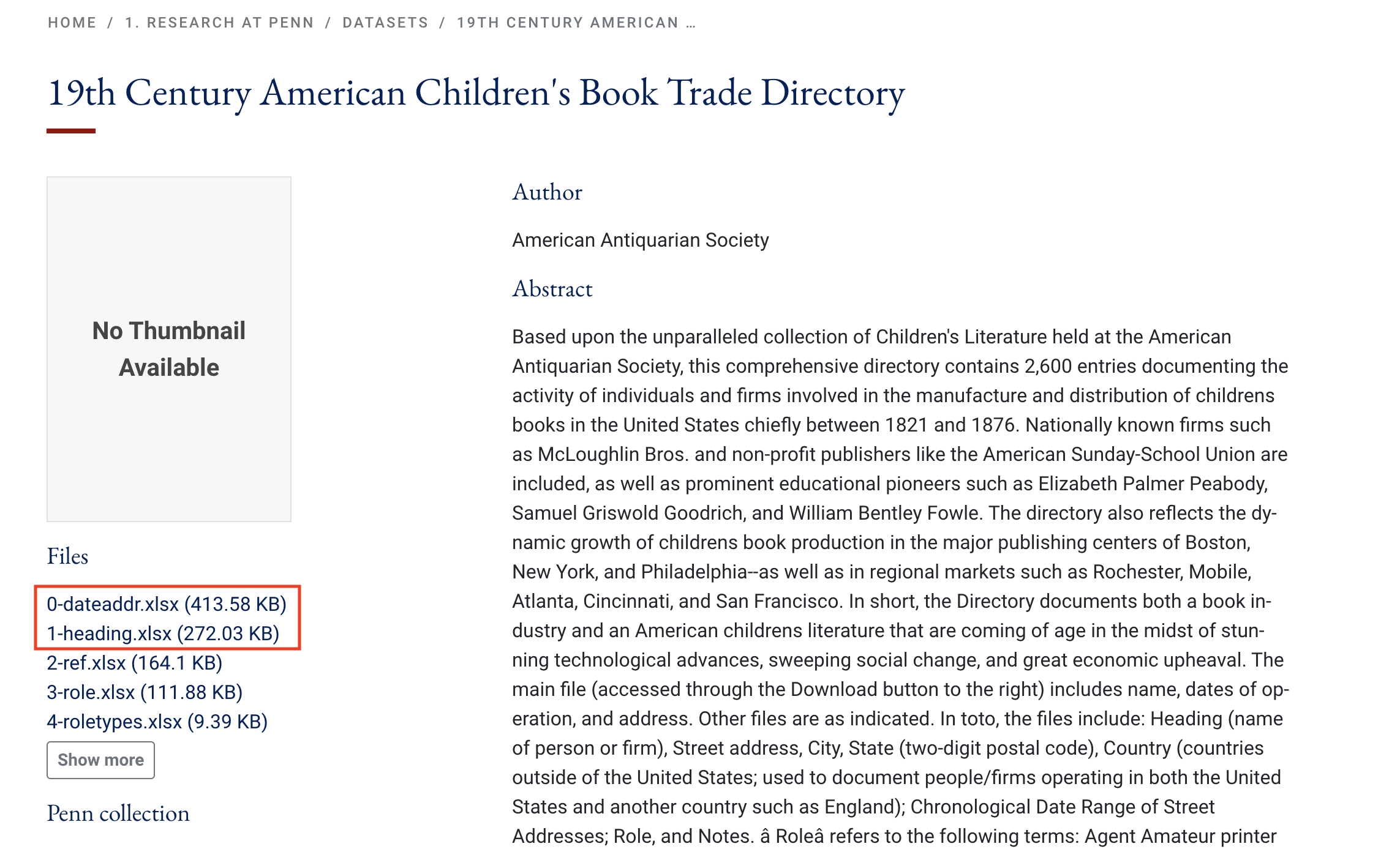
Get the data of the 19th century American children’s book trade directory from the University of Pennsylvania Scholarly Commons: https://repository.upenn.edu/entities/dataset/16705c2f-023b-495e-baf4-dee805eae59f

You should download both 0-dateaddr.xlsx and 1-heading.xlsx.

Take a beat to open the data in Microsoft Excel. Consider: which one of these files would you want to geocode?

Pre-processing

Perhaps obviously, we’re going to geocode the 0-dateaddr.xlsx file, because it contains well-structured address data. But before you geocode this data, it needs a little bit of pre-processing.

There are thousands of records in this spreadsheet. Even a fraction of this will take a while to geocode, so let’s focus on a smaller geography, like the state of Massachusetts. To do that we’re going to filter the spreadsheet and exclude all records that aren’t located in the state of Massachusetts.

In Microsoft Excel, open the 0-dateaddr.xlsx file
In the “Home” tab, click “Filter”—you should see drop-down arrows appear next to all the fields

sort
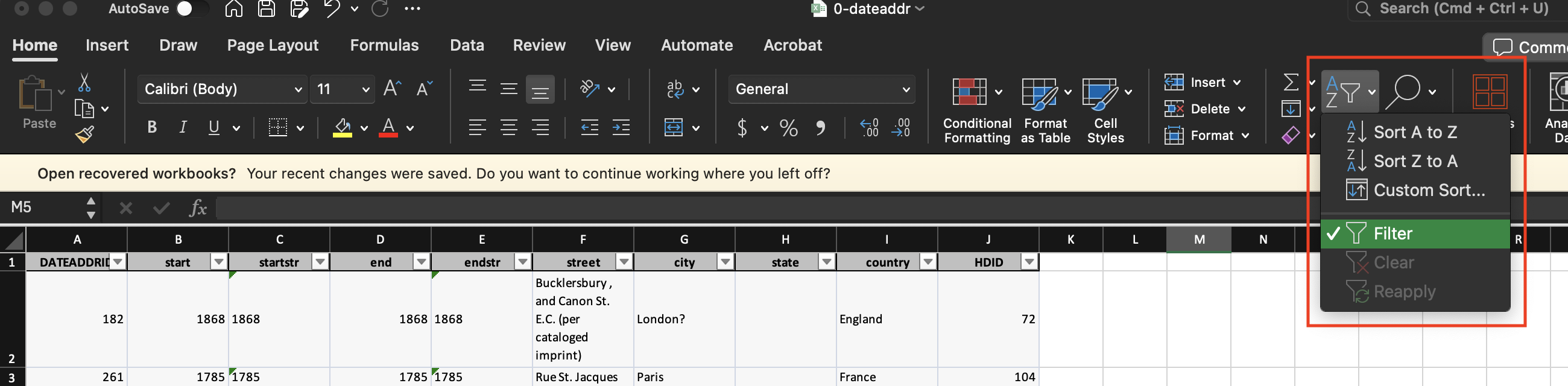
Click on the drop-down arrow by the state field ➡️ uncheck “Select All” ➡️ scroll down to “MA” and check it
Open a new spreadsheet and save it as directoryAddresses_MA. Make sure to save it as a .csv!
In 0-dateaddr.xlsx
1. select all the data with ctrl+A or another selection method of your choosing
2. copy all the data with ctrl+C or right-click ➡️ “Copy”
In directoryAddresses_MA.csv, click on the cell in the most upper left part of the spreadsheet and paste the data with ctrl+V or right-click ➡️ “Paste”
Save your spreadsheet

Now we have csv data exclusively filtered for Massachusetts—a little more manageable for this activity.

Geocoding children’s book publishers

As we discussed in class, geocoding—the process of turning descriptive address information into spatial data—requires at least two points of reference:

A topologically sound network of vector data that ideally includes things like parcel boundaries, streets, and even buildings
Descriptive information associated with that topological network, e.g., a gazetteer

Thanks to OpenStreetMap, Nominatim, and MMQGIS, we have all of these things built into QGIS for free. That’s why we’re using this instead of ArcGIS Pro: in order to geocode addresses in ArcGIS Pro, we need to pay for it. I don’t want to spend thousands of our limited ArcGIS Online credits on a learning exercise, so we’re making lemons out of lemonade and also learning a new software while we geocode for free instead.

OpenStreetMap, Nominatim, and MMQGIS

This week’s activity hinges on three pieces of software. All open source!

You already know what OpenStreetMap (OSM) is from the parking lot cemetery assignment: it’s a free and open-source base map, the “Wikipedia of maps,” because anybody can edit it. This serves as our topologically sound network of vector data as well as our descriptive information or gazetteer.
Nominatim is a free and open-source tool for geocoding with OSM data. You could geocode with Nominatim in ArcGIS Pro, but it requires writing bespoke code into the Python console.
MMQGIS is a QGIS plugin for manipulating vector map layers in Quantum GIS: CSV input/output/join, geocoding, geometry conversion, buffering, hub analysis, simplification, column modification, and simple animation. It comes installed with QGIS in all the Data Lab computers, but if you don’t see it in the toolbar at the top of your screen, it’s really easy to install (Plugins ➡️ Manage and install plugins ➡️ search for mmqgis, click it, and click “Install”).

Running the geocoder

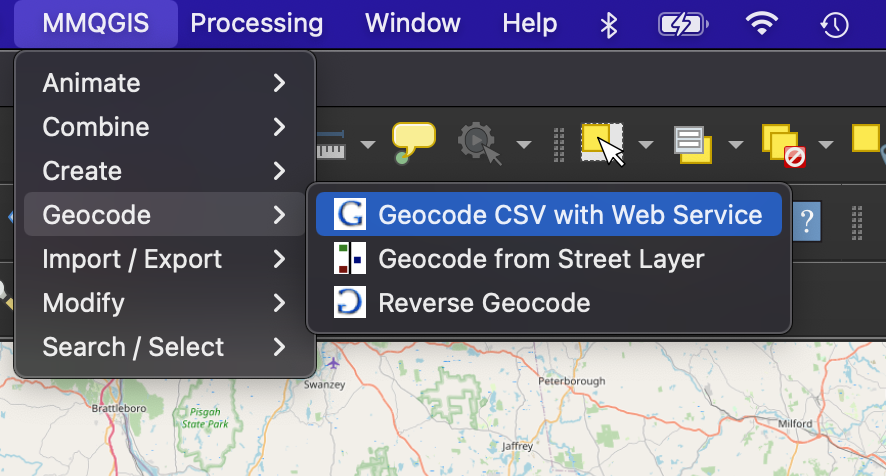
To geocode the data, navigate to the menu bar at the top of the screen and click “MMQGIS” ➡️ “Geocode” ➡️ “Geocode CSV with Web Service.” MMQGIS should appear on the upper right-hand side.

In the geocoding dialog that opens, you should see a dialog box like this:

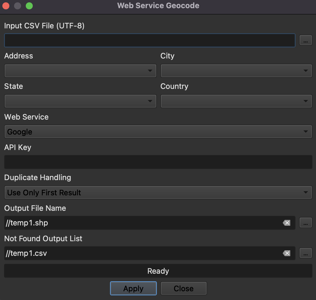
Click the little backspace arrows in the fields for “Output File Name” and “Not Found Output List.” This will make placing the output files in your workspace much easier.

Now fill out the parameters as in the image below, taking care to…

Click the backspace buttons highlighted in yellow to remove the default file paths before you
Click the ellipses highlighted in red to select

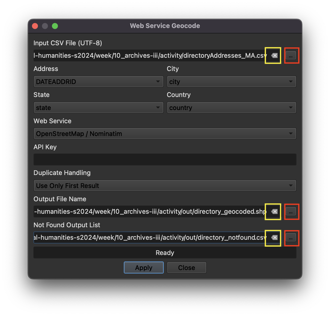
… and before you click “Apply,” make sure that the “Web Service” parameter is set to OpenStreetMap / Nominatim!

Before you click “Apply,” note that it’s probably going to take at least 15-30 minutes to fully geocode this query. It’s not a fast tool. Only run it when you have time to let it run fully.

When you’re ready, click “Apply,” and wait…

When it’s done, your geocoding dialog should see something like this:

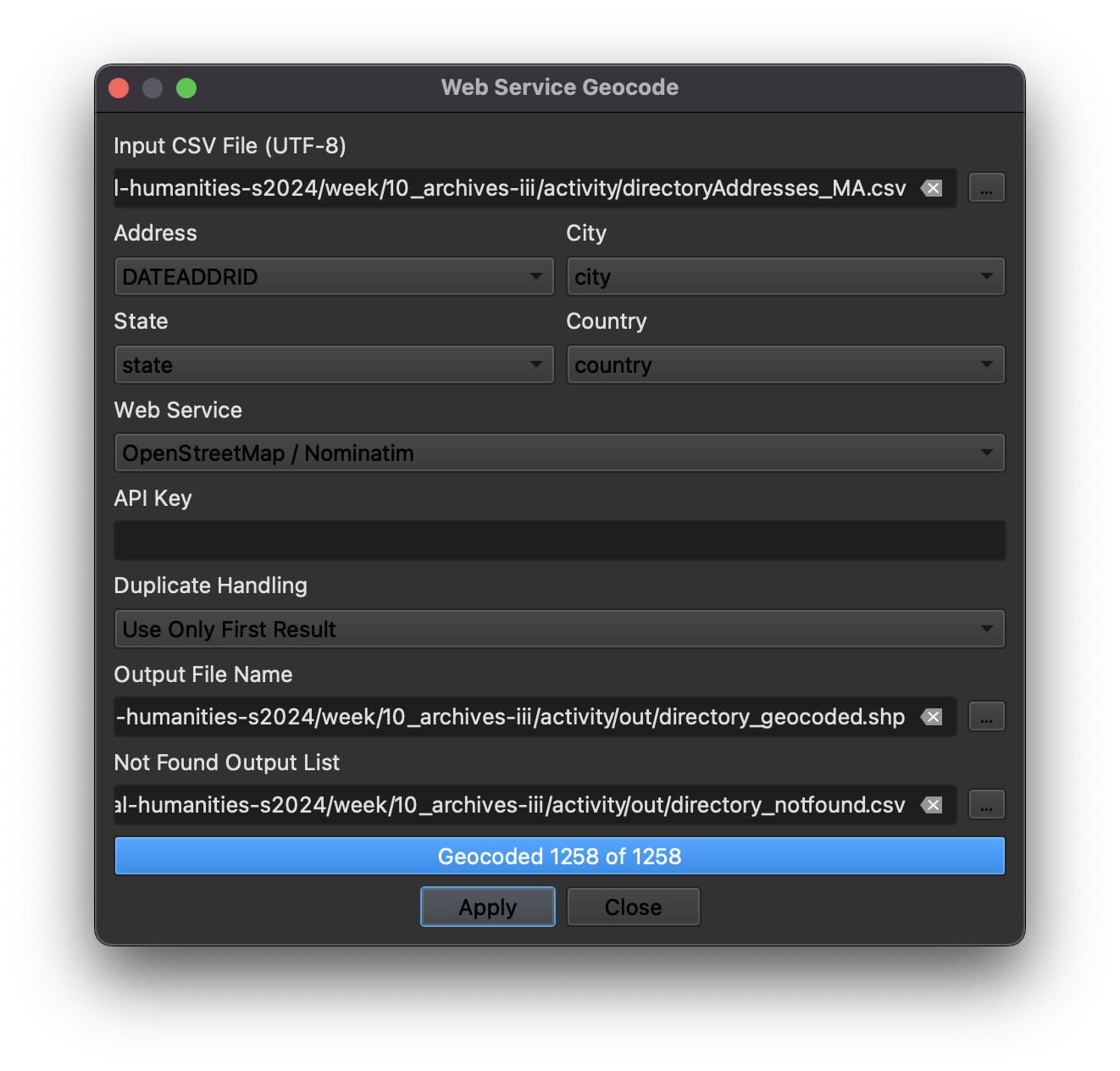
Wow! Pretty impressive that 100% of the records geocoded. Let’s exit this dialog box and go back to the map. “Right-click” the layer in your layers list—mine is titled directory_geocoded—and click “Zoom to Layer(s).” You should see something like this:

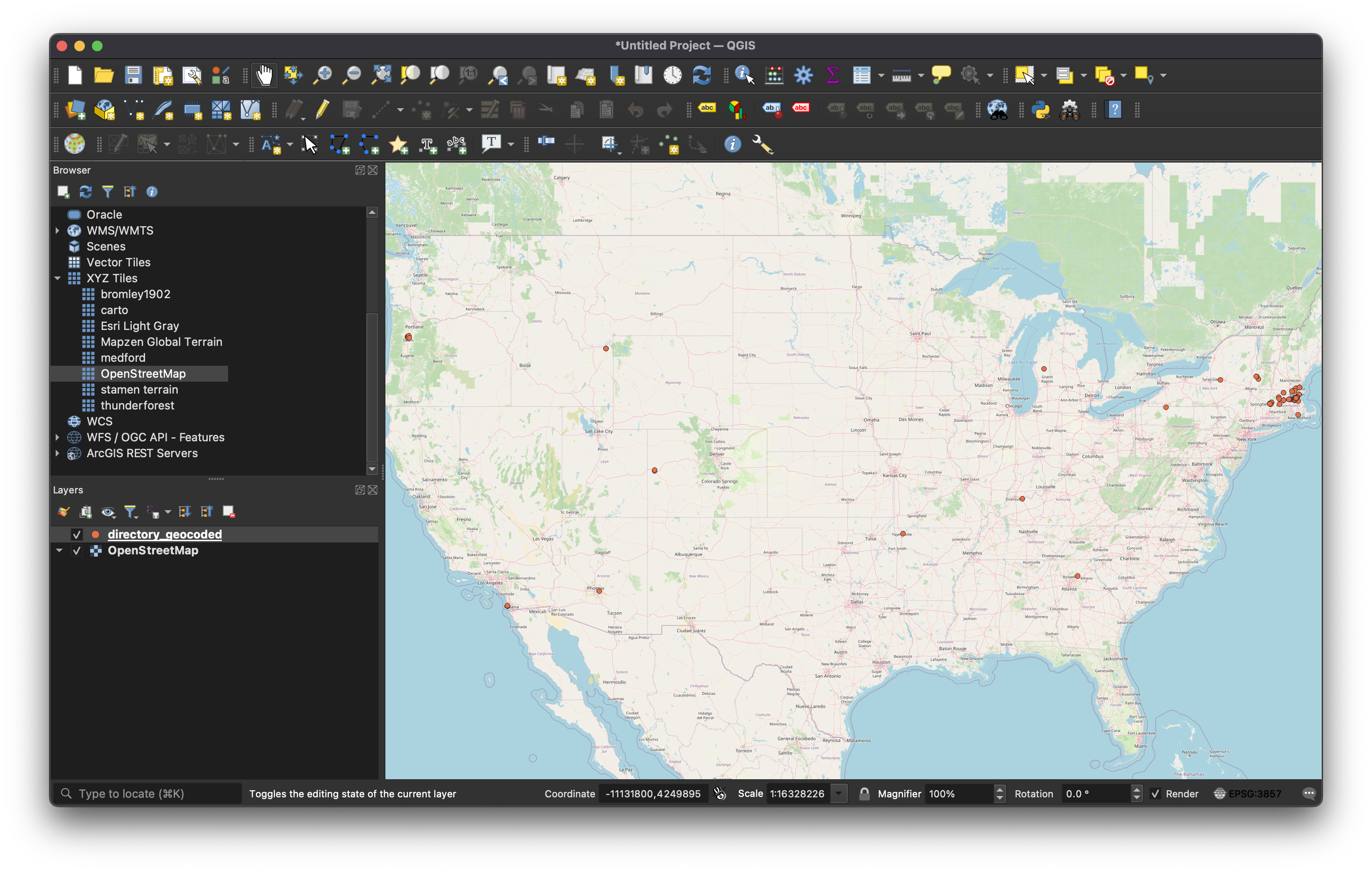
Hmmm… why did a bunch of these layers end up outside of Massachusetts?

Natural language processing “by hand”

We’re not actually going to do any computational natural language processing (NLP) in this class, but if you think about it, geocoding is itself a kind of NLP: we’re taking descriptive address data, “tokenizing” it into discrete parts, and passing that through an algorithm that can recognize those parts and assign them to places in the real world.

To wrap up this activity, I want you to do some natural language processing, but “by hand.” By this, I mean you are going to manually look through the attribute table of the geocoded data and figure out why some things ended up in places where they weren’t supposed to. This is exactly the kind of work that NLP can automate, but for now, you’re going to do a snippet of it manually.

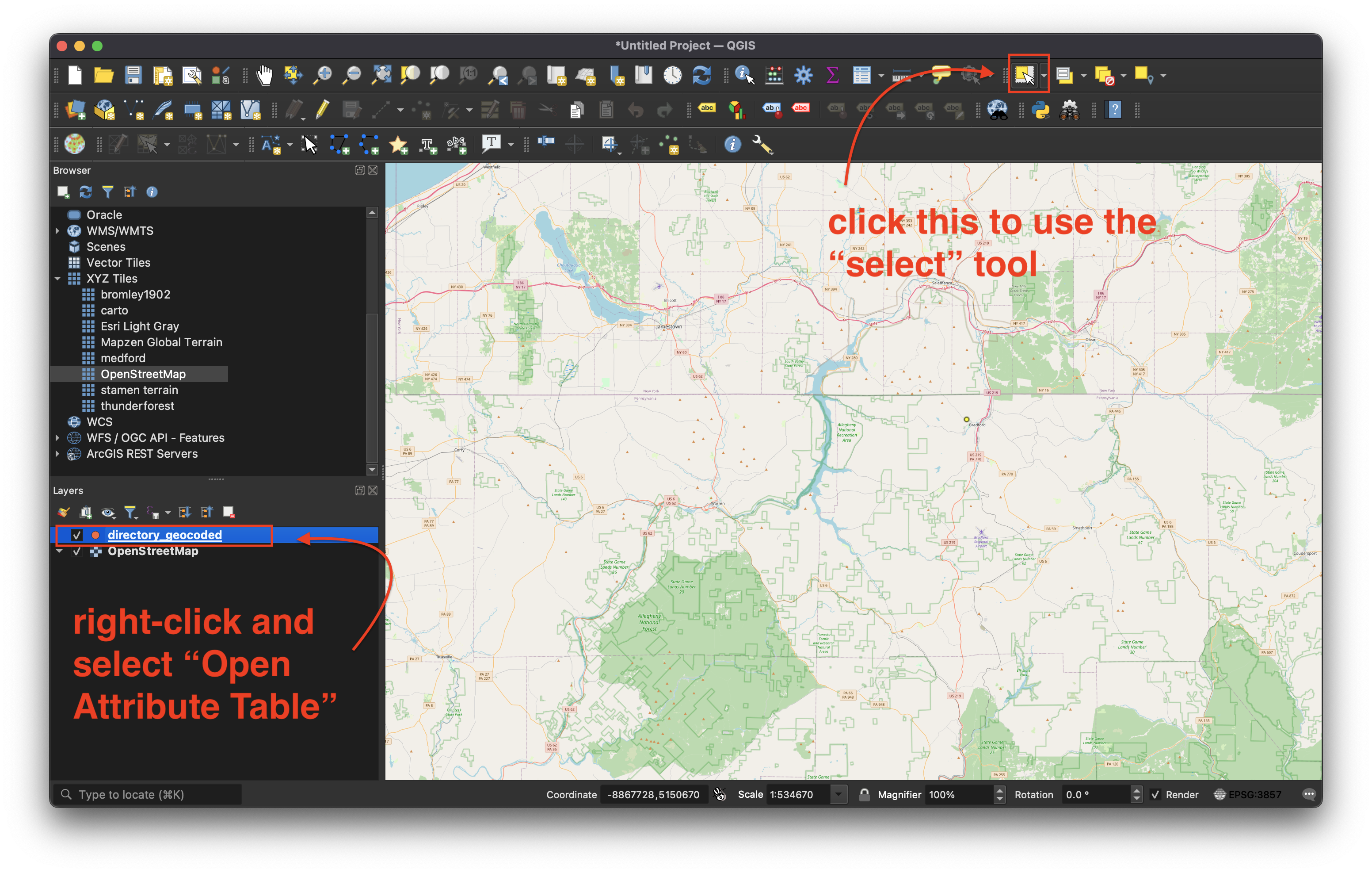
To accomplish this, you’ll need to use the selection tool and the attribute table. Both of these should feel familiar, but in QGIS, they’re just in slightly different places:

Pick five addresses from your geocoded layer and try to figure out why OSM couldn’t match them to their expected geography in Massachusetts. Consider: does the historical address, as it’s listed in the source spreadsheet, still exist? Has the address possibly changed? To figure this out, I recommend searching for the addresses as they appear in the attribute table in Google Maps. You can also try going to OSM and navigating to where you would expect that address to appear. See if you can determine why it didn’t join, and for each record, explain why you think it didn’t match, and how you think you might fix it. (These answers might be similar for multiple addresses.)

Table join to your geocoded layer

In your workspace, you should have a secondary table that you could join to the geocoded layer based on a common field.

Before trying to join anything, make sure that you save the xlsx file as a csv file. csv files behave better with QGIS.

Table joins in QGIS are pretty easy. Try following this tutorial to join the 1-heading.csv layer to your geocoded data.

You should be able to identify the common field required for the join by comparing the attribute table of your geocoded layer with the 1-heading.csv spreadsheet.

Symbolize your data

To wrap up, try symbolizing your data. It’s pretty similar in QGIS to how you’d to it in ArcGIS Pro.

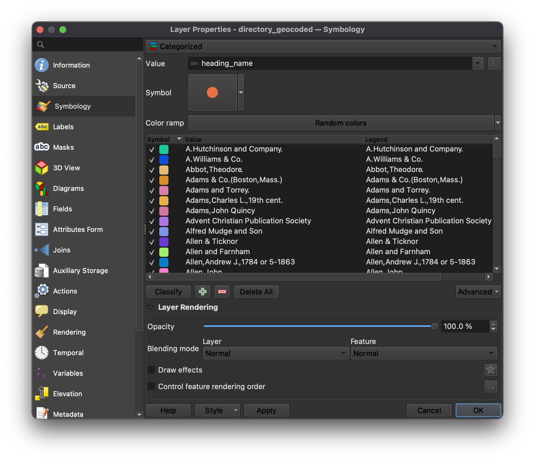
Right-click on the geocoded layer in your layers list
Click on the “Symbology” tab on the left-hand side
Pick “Categorical”
Set the value to heading_name
Click the symbol and make it bigger—maybe 4.0 in size
Use a “Random color” ramp
Click “Classify” just below the ramp
When you’re done, click “OK” in the bottom right-hand corner of the Symbology dialog

Activity deliverables

Submit